[See ref 2, ref 3]
The infinity of conceivable triplet distributions.
Chargaff's second parity rule specifies only that the numbers of triplets are equal to the numbers of their reverse complements
in every sufficiently long genomic DNA strand. But it does not specify the numbers of each triplet.
In fact, there is an infinity of possible triplet distributions, that all fulfill the rule and, yet, are all different from each other.
This is easy to show. There are 64 different triplets. They can be divided into 2 groups where the members of one group
are the reverse complements of the members of the other. For example, one such division could consist of the following groups.
GROUP 1:AGT, ATT, CAT, CCT, CGG, CGT, CTG, CTT, GAA, GAG, GAT, GCA, GCG, GCT, GGA, GGC, GGG, GGT, GTA, GTC, GTG, GTT, TAG, TAT, TCG, TCT, TGA, TGG, TGT, TTA, TTG, TTT.
GROUP 2:ACT, AAT, ATG, AGG, CCG, ACG, CAG, AAG, TTC, CTC, ATC, TGC, CGC, AGC, TCC, GCC, CCC, ACC, TAC, GAC, CAC, AAC, CTA, ATA, CGA, AGA, TCA, CCA, ACA, TAA, CAA, AAA
It is easy to verify that the groups have no triplet in common, but together make up all 64 triplets.
Now pick randomly 32 numbers that add up to 1/2, e.g.
0.024,
0.003,
0.018,
0.019,
0.011,
...
and assign them as frequencies to each member of Group 1 and the same number to the reverse complement of the same member in Group 2:
f(AGT) = f(ACT) = 0.024,
f(ATT) = f(AAT) = 0.003,
f(CAT) = f(ATG) = 0.018,
f(CCT) = f(AGG) = 0.019,
f(CGG) = f(CCG) = 0.011,
...
The resulting frequency distribution will, by way of its construction, be normalized and fulfil Chargaff's second parity rule perfectly.
The choice of the 32 numbers was completely arbitrary and, therefore, there is an infinity of such choices. Consequently, there is an
infinity of different conceivable triplet distributions.
There is also an infinity of DNA sequences that have any of these as their frequency distributions. Say, you want a DNA sequence of 3 Mb
length and the exact triplet distribution of the above example. Just multiply each the above numbers by 1000,000 and take as many triplets, i.e.
24,000 AGT's and 24,000 ACT's,
3000 ATT's and 3000 AAT's,
18,000 CAT's and 18,000 ATG's,
19,000 CCT's and 19,000 AGG's,
11,000 CGG's and 11,000 CCG's,
...
and let a computer mix up their order randomly. The result will be an unpredictable sequence of nucleotides with the exact frequency distribution
of the above example and 3 Mb size.
In short, one should expect that different genomes, although all complying with the
symmetry rule, have quite different triplet distributions.
The actual number of triplet distributions: only 3(!)
Measuring the triplet profiles of 31 chromosomes of different organisms ranging from rickettsia to humans, including human, chimpanzee,
mouse, zebrafish, maize, streptococcus pneum.,Arabidopsis, xenopus laevis, yeast, B. subtilis, anopheles, and others yielded the
surprising result that all of these very different organisms had effectively the same triplet distribution (Fig.1). I suggest to call the distribution the 'majority
distribution' and their class the 'majority class'.
There are also 2 other classes with much fewer members including the class of mitochondrial genomes that violate intra-strand symmetry.They are described
in more detail in ref 2. The present chapter will focus on the majority profile and the majority class.
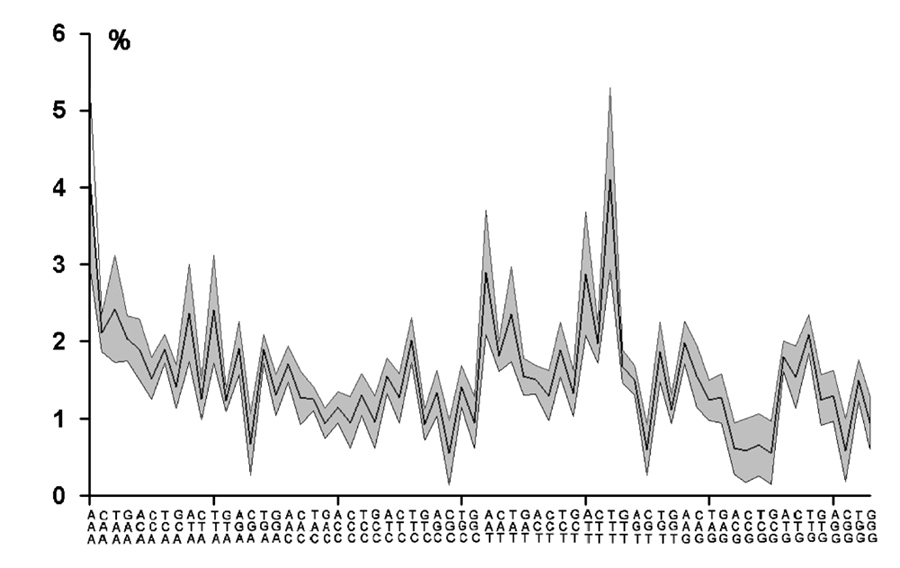
Fig.1. Majority triplet profile (Abscissa: triplets to be read from bottom to top; Ordinate: fraction of triplets
of entire genome).
The shaded area covers the range of the standard deviation computed from the triplet profiles of 31 chromosomes
of different organisms ranging from rickettsia to humans, including human, chimpanzee, mouse, zebrafish, maize, streptococcus pneum.,
Arabidopsis, xenopus laevis, yeast, B. subtilis, anopheles, and others.
As illustrated in Fig.2, the majority profile, of course, obeys Chargaff's second parity rule. However, in view of the infinity of conceivable triplet distributions the it poses the burning question, how it is possible that such different organisms
ended up having the same triplet distribution.
Especially disturbing is the fact that we know of no selective advantage associated with genomes having
one or the other of the described types of triplet profiles. There is not even a known selective advantage associated with the much less stringent
condition of a genome's compliance with Chargaff's second parity rule. Yet, both these conditions appear to be almost universally fulfilled by genomes.
In the past, the most useful guide in the interpretation of genome properties was the phylogenetic position of the organism in question. Unfortunately,
this approach must fail in the case of a genome's compliance with Chargaff's second parity rule, or its particular class of triplet profile, because
both properties seem to have no phylogenetic correlation.
It seems possible, though, to assume that all these genomes had the same beginning and, as they evolved into very different sequences, the same
'functional anarchy' of mutations molded their sequence structure and architecture into closely related 'shapes', as will be proposed in the following
section.
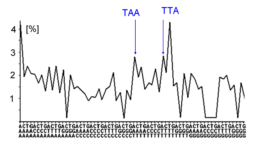
Fig.2. Compliance with inter-strand symmetry (triplet profile of Chimpanzee chr. 14, position: 32 Mb to 40 Mb). (Abscissa: all possible triplets
(to be read vertically from bottom to top). Ordinate: frequency of triplets [%]).
The blue labels show the example of the equal amplitude of the TAA triplet and its reverse complement, AAT.
The hypothetical evolution of the majority profile.
STEP 1: Consistent with the ideas of the so-called "RNA-world" we assume that the initial genomes were random concatenations of 4 nucleotides that reflected their
initial concentrations in the initial 'soup'. We assume as initial concentrations p0(A) = 0.20, p0(T) = 0.36, p0(C) = 0.25, p0(G) = 0.19. As shown in
ref 3, the actual numbers are not very critical, but they should be in the range given here.
If the concatenation into polymers was, indeed, random, one would expect that the probabilty p(XYZ) of a triplet XYZ, would be given by
p(XYZ) = p(X)p(Y)p(Z).
Figure 3a shows how the resulting triplet distribution would look. Of course, it does not obey the intra-strand symmetry, as not even the numbers of the
complementary bases are equal: p(A)≠p(T) and p(C)≠p(G).
STEP 2:The next step is an ad hoc reconstruction. It assumes that a global event occurred that changed 60% of CG dinucleotides int TT dinucleotides.
The arguments concerning this step are discussed in ref 3. Even though a conversion rate of 60 % may
sound like a large modification, the number of sequence alterations was actually rather small. Using the base composition of the above equation, the
stochastic-expectation genomes of Fig. 3a contained approximately 5% CG pairs on either strand. Therefore, the required sequence changes involved
only 3% modification of their total di-nucleotides. Figure 3b shows how this second step altered the triplet distributions. Its main effect was to
increase the number of TTT triplets substantially. The resulting distribution still violated the intra-strand symmetry massively.
STEP 3:As a last step we unleash the same large number of inversions/inverted transpositions that were used in the previous chapter to achive the
intra-strand symmetry. As shown in in Figure 3c, this process not only generated the strand symmetry, but created a triplet profile that was almost identical to the majority profile
(cCW = 0.957). Figure 3d shows the close similarity by superimposing the majority profile in red with the profile of Fig. 3c.

Fig.3. The majority profile as the result of numerous inversions/inverted transpositions.
( Abscissa: triplets to be read from bottom to top; Ordinate: fraction of triplets of entire genome).
a. Random expectation: Let T = XYZ be a triplet, then p(T) = p(X)p(Y)p(Z) ('urn experiment with replacement'). In this simplest case the
simulation uses the nucleotide frequencies p0(A) = 0.20, p0(T) = 0.36, p0(C) = 0.25, p0(G) = 0.19. (NOTE: The frequencies are arbitrary and
do not comply with Chargaff's second parity rule).
b. Effect of replacing randomly 60% of all CG pairs with TT pairs.
c. Effect of 30,000 inversions/transpositions of 1 kb size on the triplet profile of the simulated genome of Panel b.
d. Superimposition of the majority profile (red) and the simulated profile of panel c. (correlation coefficient between the two profiles is 0.957).
The quite understandable mechanism of profile conversion.
The conversion of the profile of Fig. 3b to the majority profile was carried out by a computer program. However, no computer is needed for that.
As shown earlier, the large number of inversions/inverted transpositions does nothing more than turn the initally different frequencies of a triplet and its
reverse complement into a common value, namely their arithmetic mean. This is illustrated in Figure 4.So, in order to effect the conversion, one would need
no more than a ruler and a calculator. Then one would measure the amplitudes of each triplet and its reverse complement in Figure 3b, form the arithmetic mean
and plot it as the new amplitude of both.
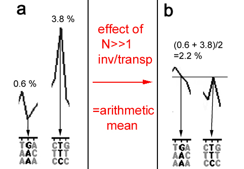
Fig.4. The effect of numerous of inversions/transpositions needs no computer: It is simply the formation of the arithmetic mean between the initial
frequencies of each triplets and its reverse complements (see Fig.5 of previous chapter where the frequencies of the 2
complimentary nucleotides G and C converge to
their arithmetic mean (labeled "theoretical")). The examples of the triplet AAG and its reverse complement CTT shown here were excised from
Figures 2b and 2c and printed to scale.
a. Initial frequencies of AAG and CTT before any inversions/transpositions.
b. Equalized final frequencies of the same 2 triplets after 30,000 inversions/transpositions representing the arithmetic mean of the initial values.
General implications of the existence of the majority profile
Every organism with the majority profile obeys, in particular,
Chargaff's second parity rule. Therefore, all the mentioned consequences of this strand symmetry, such as
the the equalisation of physical properties of the strands,
the asymptotic progress towards perfection ,
the invariance against the major other mechanisms of variation, and
the difficulty to identify a selective advantage are also consequences
of the majority profile.
But clearly, the existence of the majority profile goes considerably beyond the condition that the counts of every
triplet are the same on the Watson- and the Crick-strand for so many very different organisms. Since their distributions
are the same, it means that these counts are proportional to the genome (chromosome) size. In other words, if the genome of
an organism is twice as large than that of another, their triplet counts are twice as large as well.
Does the majority profile facilitate horizontal gene transfer?
Again the question arises whether the commonality of the distributions of so many different genomes constitutes a selective advantage?
In contrast to the previously stated doubts, in this case one may speculate it may
facilitate horizontal gene transfer between vastly different species as their common triplet distributions may have rendered native and foreign sequences, especially the non-coding parts of genes,
similar enough, at least locally, to be inserted and/or exchanged. In this way it may speed up evolution considerably, as horizontal gene
transfer makes it unnecessary for different organisms to re-invent the same beneficial genes many times over.
Is the evolutionary appearance of new orders linked to local changes of triplet distributions of the common ancestor?
There seems to exist an even deeper implication of the the existence of the majority profile. As will be shown in a later chapter ('signatures'), the local deviations of genomes from the majority
profile are highly conserved within the members of an order, as if their first appearance identified an organism as the founder of a new order.